python sklearn でロジスティック回帰。fit して predict、引数 C で正則化

簡単なデータでロジスティク回帰を試してみます。やるのは２クラスの分類ですが、理論的なことはとりあえず置いといて、 python の scikit-learnライブラリを使ってみます。このライブラリの
LogisticRegression というクラスがロジスティック回帰です。

メソッド fit、predict、score、属性 coef_、intercept_、パラメータ C を使ってみました。

- 目次 -

データ
訓練
プロット
C を指定
C は正則化のパラメータ

データ

データとして、二次元正規分布のかたまりを 2 組つくっておきます。

from sklearn.cross_validation import train_test_split
from sklearn.preprocessing import StandardScaler
import matplotlib.pyplot as plt
import numpy as np

np.random.seed(seed=0)
X_0 = np.random.multivariate_normal( [2,2],  [[2,0],[0,2]],  50 )
y_0 = np.zeros(len(X_0))

X_1 = np.random.multivariate_normal( [6,7],  [[3,0],[0,3]],  50 )
y_1 = np.ones(len(X_1))

X = np.vstack((X_0, X_1))
y = np.append(y_0, y_1)

X_train, X_test, y_train, y_test = train_test_split(X, y, test_size=0.3)

# 特徴データを標準化(平均 0、標準偏差 1)
sc = StandardScaler()
X_train_std = sc.fit_transform(X_train)
X_test_std = sc.transform(X_test)

plt.scatter(X_train_std[y_train==0, 0], X_train_std[y_train==0, 1], c='red', marker='x', label='train 0')
plt.scatter(X_train_std[y_train==1, 0], X_train_std[y_train==1, 1], c='blue', marker='x', label='train 1')
plt.scatter(X_test_std[y_test==0, 0], X_test_std[y_test==0, 1], c='red', marker='o', s=60, label='test 0')
plt.scatter(X_test_std[y_test==1, 0], X_test_std[y_test==1, 1], c='blue', marker='o', s=60, label='test 1')

plt.legend(loc='upper left')

from sklearn.cross_validation import train_test_split

from sklearn.preprocessing import StandardScaler

import matplotlib.pyplot as plt

import numpy as np

np.random.seed(seed=0)

X_0 = np.random.multivariate_normal( [2,2], [[2,0],[0,2]], 50 )

y_0 = np.zeros(len(X_0))

X_1 = np.random.multivariate_normal( [6,7], [[3,0],[0,3]], 50 )

y_1 = np.ones(len(X_1))

X = np.vstack((X_0, X_1))

y = np.append(y_0, y_1)

X_train, X_test, y_train, y_test = train_test_split(X, y, test_size=0.3)

# 特徴データを標準化(平均 0、標準偏差 1)

sc = StandardScaler()

X_train_std = sc.fit_transform(X_train)

X_test_std = sc.transform(X_test)

plt.scatter(X_train_std[y_train==0, 0], X_train_std[y_train==0, 1], c='red', marker='x', label='train 0')

plt.scatter(X_train_std[y_train==1, 0], X_train_std[y_train==1, 1], c='blue', marker='x', label='train 1')

plt.scatter(X_test_std[y_test==0, 0], X_test_std[y_test==0, 1], c='red', marker='o', s=60, label='test 0')

plt.scatter(X_test_std[y_test==1, 0], X_test_std[y_test==1, 1], c='blue', marker='o', s=60, label='test 1')

plt.legend(loc='upper left')

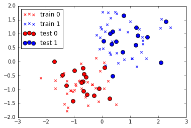
区分が 0 のデータを 50個、1 のデータを 50個 用意し、訓練データとテストデータを 7:3 に分割します。

下記はプロット結果。× が 訓練データ、○ が テストデータ です。

訓練

訓練は LogisticRegression のメソッド fit にデータを渡すだけです。

from sklearn.linear_model import LogisticRegression

# 訓練
lr = LogisticRegression()
lr.fit(X_train_std, y_train)

from sklearn.linear_model import LogisticRegression

# 訓練

lr = LogisticRegression()

lr.fit(X_train_std, y_train)

訓練終了。

では、訓練したモデルにテストデータを当てはめてみます。分類は predict、精度の確認は score メソッドで行います。

# テストデータ 30個を分類
print (lr.predict(X_test_std))
#-------------------------------------------------------------------------
# [ 0.  0.  0.  1.  1.  0.  0.  1.  0.  0.  1.  0.  1.  1.  1.  0.  1.  1.
#   1.  1.  1.  0.  0.  0.  0.  0.  0.  0.  0.  1.]
#-------------------------------------------------------------------------

# 精度を確認
print (lr.score(X_test_std, y_test))
#----------------
# 0.966666666667
#----------------

# テストデータ 30個を分類

print (lr.predict(X_test_std))

#-------------------------------------------------------------------------

# [ 0. 0. 0. 1. 1. 0. 0. 1. 0. 0. 1. 0. 1. 1. 1. 0. 1. 1.

# 1. 1. 1. 0. 0. 0. 0. 0. 0. 0. 0. 1.]

#-------------------------------------------------------------------------

# 精度を確認

print (lr.score(X_test_std, y_test))

#----------------

# 0.966666666667

#----------------

精度は 96.7 %。残念ながら 100 % に届きませんでしたが、この精度はパラメータ C を指定することで変化します（後述）。

プロット

ロジスティック回帰の訓練結果は境界線

\(w_0+w_1x+w_2y=0\)

の重み \(w_0\)、\(w_1\)、\(w_2\)ですが、その値は属性 intercept_、coef_ に入っています。値を取得し、境界線をプロットしてみます。

print (lr.intercept_)
#-----------------------------
# [ 0.13310259]
#-----------------------------

print (lr.coef_)
#-----------------------------
# [[ 1.82092295  2.26785197]]
#-----------------------------

w_0 = lr.intercept_[0]
w_1 = lr.coef_[0,0]
w_2 = lr.coef_[0,1]

# 
# 境界線の式
#   w_1・x + w_2・y + w_0 = 0
#   ⇒ y = (-w_1・x - w_0) / w_2

# 境界線 プロット
plt.plot([-2,2], map(lambda x: (-w_1 * x - w_0)/w_2, [-2,2]))

# データを重ねる
plt.scatter(X_train_std[y_train==0, 0], X_train_std[y_train==0, 1], c='red', marker='x', label='train 0')
plt.scatter(X_train_std[y_train==1, 0], X_train_std[y_train==1, 1], c='blue', marker='x', label='train 1')
plt.scatter(X_test_std[y_test==0, 0], X_test_std[y_test==0, 1], c='red', marker='o', s=60, label='test 0')
plt.scatter(X_test_std[y_test==1, 0], X_test_std[y_test==1, 1], c='blue', marker='o', s=60, label='test 1')

print (lr.intercept_)

#-----------------------------

# [ 0.13310259]

#-----------------------------

print (lr.coef_)

#-----------------------------

# [[ 1.82092295 2.26785197]]

#-----------------------------

w_0 = lr.intercept_[0]

w_1 = lr.coef_[0,0]

w_2 = lr.coef_[0,1]

# 境界線の式

# w_1・x + w_2・y + w_0 = 0

# ⇒ y = (-w_1・x - w_0) / w_2

# 境界線プロット

plt.plot([-2,2], map(lambda x: (-w_1 * x - w_0)/w_2, [-2,2]))

# データを重ねる

plt.scatter(X_train_std[y_train==0, 0], X_train_std[y_train==0, 1], c='red', marker='x', label='train 0')

plt.scatter(X_train_std[y_train==1, 0], X_train_std[y_train==1, 1], c='blue', marker='x', label='train 1')

plt.scatter(X_test_std[y_test==0, 0], X_test_std[y_test==0, 1], c='red', marker='o', s=60, label='test 0')

plt.scatter(X_test_std[y_test==1, 0], X_test_std[y_test==1, 1], c='blue', marker='o', s=60, label='test 1')

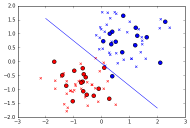
精度が 96.7 %でしたが、確かに、テストデータ 30個のうち 1個のデータ（青丸）が境界線をはみ出しています。

C を指定

C を指定することで精度が変化すると書きました。実際にやってみます。C はデフォルトで 1.0 とされており、ここでは 10、100、1000 で試してみます。

fig, axs = plt.subplots(2, 2, sharex=True, sharey=True)
plt.ylim([-2, 2])
plt.subplots_adjust(wspace=0.1, hspace=0.6)
c_params = [1.0, 10.0, 100.0, 1000.0]
for i, c in enumerate(c_params):
    lr = LogisticRegression(C=c)
    lr.fit(X_train_std, y_train)

    w_0 = lr.intercept_[0]
    w_1 = lr.coef_[0,0]
    w_2 = lr.coef_[0,1]
    score = lr.score(X_test_std, y_test)

    axs[i/2, i%2].set_title('C=' + str(c))
    axs[i/2, i%2].plot([-2,2], map(lambda x: (-w_1 * x - w_0)/w_2, [-2,2]))

    axs[i/2, i%2].scatter(X_train_std[y_train==0, 0], X_train_std[y_train==0, 1], c='red', marker='x', label='train 0')
    axs[i/2, i%2].scatter(X_train_std[y_train==1, 0], X_train_std[y_train==1, 1], c='blue', marker='x', label='train 1')
    axs[i/2, i%2].scatter(X_test_std[y_test==0, 0], X_test_std[y_test==0, 1], c='red', marker='o', s=60, label='test 0')
    axs[i/2, i%2].scatter(X_test_std[y_test==1, 0], X_test_std[y_test==1, 1], c='blue', marker='o', s=60, label='test 1')

    if (i < 2):
        axs[i/2, i%2].text(0,-2.7, 'score ' + str(round(score,3)*100) + '%', size=13)
    else:
        axs[i/2, i%2].text(0,-3.3, 'score ' + str(round(score,3)*100) + '%', size=13)

fig, axs = plt.subplots(2, 2, sharex=True, sharey=True)

plt.ylim([-2, 2])

plt.subplots_adjust(wspace=0.1, hspace=0.6)

c_params = [1.0, 10.0, 100.0, 1000.0]

for i, c in enumerate(c_params):

lr = LogisticRegression(C=c)

lr.fit(X_train_std, y_train)

w_0 = lr.intercept_[0]

w_1 = lr.coef_[0,0]

w_2 = lr.coef_[0,1]

score = lr.score(X_test_std, y_test)

axs[i/2, i%2].set_title('C=' + str(c))

axs[i/2, i%2].plot([-2,2], map(lambda x: (-w_1 * x - w_0)/w_2, [-2,2]))

axs[i/2, i%2].scatter(X_train_std[y_train==0, 0], X_train_std[y_train==0, 1], c='red', marker='x', label='train 0')

axs[i/2, i%2].scatter(X_train_std[y_train==1, 0], X_train_std[y_train==1, 1], c='blue', marker='x', label='train 1')

axs[i/2, i%2].scatter(X_test_std[y_test==0, 0], X_test_std[y_test==0, 1], c='red', marker='o', s=60, label='test 0')

axs[i/2, i%2].scatter(X_test_std[y_test==1, 0], X_test_std[y_test==1, 1], c='blue', marker='o', s=60, label='test 1')

if (i < 2):

axs[i/2, i%2].text(0,-2.7, 'score ' + str(round(score,3)*100) + '%', size=13)

else:

axs[i/2, i%2].text(0,-3.3, 'score ' + str(round(score,3)*100) + '%', size=13)

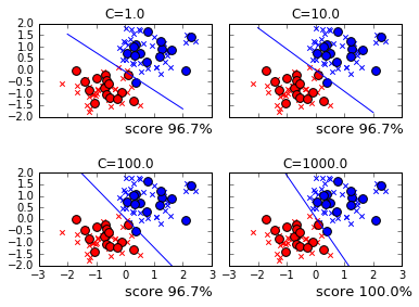
C を変化させると境界線が徐々に変化し、C=1000 で精度 100% の位置を探し当てています。以下は、それぞれの C で導き出された重みです。

C
1.0
10.0
100.0
1000.0

w_0
0.1331
0.00025
-0.35115
-0.85447

w_1
1.821
3.76
8.465
19.084

w_2
2.268
4.133
6.673
10.556

C が大きくなるにつれて w_1 と w_2 が大きくなっています。C とは一体何でしょうか？

C は正則化のパラメータ

LogisticRegression の正則化は、デフォルトの場合、L2正則化です。L2正則化では、コスト関数

\(J(\mathbf{w})=\sum_{i=1}^n \Bigl[ -y^{(i)} log \big( \phi \big(z^{(i)}\big) \big)- \big(1-y^{(i)}\big)log \big(1-\phi \big(z^{(i)} \big) \big) \Bigr] \)

に対して、正則化項

\( \large{\frac{ \lambda }{2}} \ \normalsize{\sum_{j=1}^m w^2_j} \)

が付加されます。ここで \(\lambda\) を指定して正則化の強さを指定しますが、LogisticRegression では \(\lambda\) の代わりに C を指定します。C と \(\lambda\) は

\(C=\large{\frac{1}{\lambda }}\)

の関係にあり、コスト関数はこうなります。

\(J(\mathbf{w})=\sum_{i=1}^n \Bigl[ -y^{(i)} log \big( \phi \big(z^{(i)}\big) \big)- \big(1-y^{(i)}\big)log \big(1-\phi \big(z^{(i)} \big) \big) \Bigr] +\large{\frac{1}{2\bf{C}}} \ \normalsize{\sum_{j=1}^m w^2_j}\)

C の値を大きくすると正則化が弱くなり、その結果、重みが大きくなったのが先のサンプルです。

tehqstt says:

2019年5月20日 at 2:24 AM

Спасибо за информацию!!!!!

返信
StephenNUPLE says:

2019年12月6日 at 10:41 AM

http://4092819.taf-ev.de/books-read-8822/352006-1279767391-online.html – More info!

返信
DonJat says:

2022年6月19日 at 2:11 PM

With greatest satisfaction IPTV Provider, Pronunciamento your fee today.
https://phtvmedia.com/iptv

返信

コード７区

機械学習とかpythonとか

python sklearn でロジスティック回帰。fit して predict、引数 C で正則化

データ

訓練

プロット

C を指定

C は正則化のパラメータ

3 Responses on “python sklearn でロジスティック回帰。fit して predict、引数 C で正則化”

tehqstt says:

StephenNUPLE says:

DonJat says:

コメントはお気軽にコメントをキャンセル

データ

訓練

プロット

C を指定

C は正則化のパラメータ

tehqstt says:

StephenNUPLE says:

DonJat says:

コメントはお気軽に コメントをキャンセル

コメントはお気軽にコメントをキャンセル