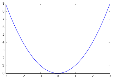
python の matplotlib でグラフを描くのは非常に簡単です。とくに、グラフが 1 つだけの場合は
|
1 2 3 4 5 6 7 8 |
import matplotlib.pyplot as plt import numpy as np x = np.linspace(-3, 3, 20) y = x ** 2 plt.plot(x, y) plt.show() |
と、わずかな記述だけで描画が実行されます。
グラフが複数の場合は少しだけ考慮が必要になるので、それを順に見ていきます。
複数のグラフ
複数のグラフを描く場合figureとaxesという概念が出てきます。figure は図全体、axes はその内部に用意される座標軸です。
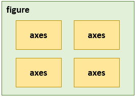
figure – axes
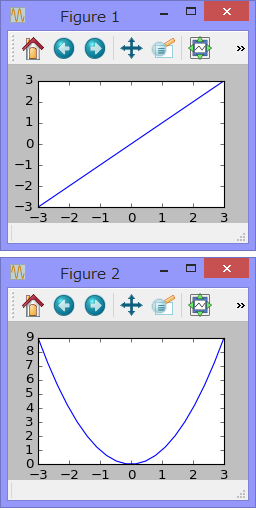
実際にグラフを 2 つ描く場合は
- figureを 1 つ用意し、その中にaxesを 2 つ作成するケース
- figureを 2 つ用意し、その中にaxesを 1 つづつ作成するケース
が考えられます。
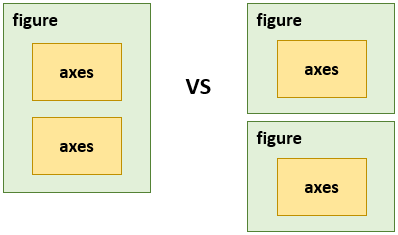
それぞれのサンプルはこうなります。
|
1 2 3 4 5 6 7 8 9 10 11 12 13 14 |
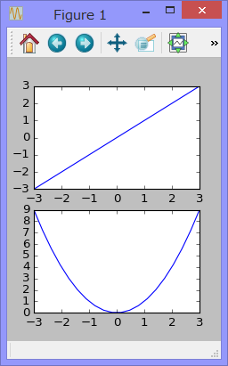
x = np.linspace(-3, 3, 20) y1 = x y2 = x ** 2 # figure は 1 つ plt.figure(figsize=(3, 4)) plt.subplot(2,1,1) plt.plot(x, y1) plt.subplot(2,1,2) plt.plot(x, y2) plt.show() |
|
1 2 3 4 5 6 7 8 9 10 11 12 13 14 |
x = np.linspace(-3, 3, 20) y1 = x y2 = x ** 2 # figure 1 つ目 plt.figure(figsize=(3, 2)) plt.plot(x, y1) # figure 2 つ目 plt.figure(figsize=(3, 2)) plt.plot(x, y2) plt.show() |
figure メソッドで figure を作成、subplot メソッドで axes を作成しています(subplot メソッドについては後述します)。
描画は以下のようになります。
ファイルへの保存は figure 単位
保存はsavefigメソッドで行いますが
|
1 |
plt.savefig("image.png") |
figure 単位で保存されるので、1 ファイルにまとめたければ前者、グラフごとにわけて保存したければ後者になります。
~~~
では、ここからは figure を 1 つにして、内部に複数のグラフを描く方法を詳しく見ていきます。
subplot
グリッド上にグラフを配置
グリッド上に規則正しくグラフを配置する場合はsubplotメソッドを使います。
|
1 |
subplot(行数, 列数, プロット番号) |
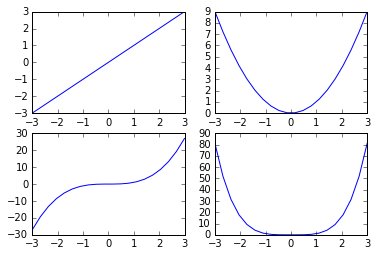
行数 × 列数 のグリッドに figure が分割され、プロット番号の位置に座標軸が作成されます。
プロット番号は、左上が 1 で、右方向、下方向へいくにしたがい値が大きくなります。たとえば、2 × 2 のグリッドの場合は
| 1 | 2 |
| 3 | 4 |
となります。
|
1 2 3 4 5 6 7 8 9 10 11 12 13 14 15 16 17 18 19 20 21 22 23 24 25 |
x = np.linspace(-3, 3, 20) y1 = x y2 = x ** 2 y3 = x ** 3 y4 = x ** 4 plt.figure(figsize=(6,4)) # 左上 plt.subplot(2,2,1) plt.plot(x, y1) # 右上 plt.subplot(2,2,2) plt.plot(x, y2) # 左下 plt.subplot(2,2,3) plt.plot(x, y3) # 右下 plt.subplot(2,2,4) plt.plot(x, y4) plt.show() |
plt.subplot(2,2,1) は カンマを省いて plt.subplot(221) と書くこともできます。ただし、プロット番号が 10 以上の場合は、カンマが必須です。
下記のとおり描画されます。
別の書き方
上記サンプルは、以下のような書き方もできます。結果は同じになります。
|
1 2 3 4 5 6 7 8 9 10 11 12 13 14 15 16 17 18 19 20 21 |
x = np.linspace(-3, 3, 20) y1 = x y2 = x ** 2 y3 = x ** 3 y4 = x ** 4 fig, axs = plt.subplots(2, 2, figsize=(6, 4)) # 左上 axs[0, 0].plot(x, y1) # 右上 axs[0, 1].plot(x, y2) # 左下 axs[1, 0].plot(x, y3) # 右下 axs[1, 1].plot(x, y4) plt.show() |
|
1 2 3 4 5 6 7 8 9 10 11 12 13 14 15 16 17 18 19 20 21 22 23 24 25 |
x = np.linspace(-3, 3, 20) y1 = x y2 = x ** 2 y3 = x ** 3 y4 = x ** 4 fig = plt.figure(figsize=(6, 4)) # 左上 ax1 = fig.add_subplot(2, 2, 1) ax1.plot(x, y1) # 右上 ax2 = fig.add_subplot(2, 2, 2) ax2.plot(x, y2) # 左下 ax3 = fig.add_subplot(2, 2, 3) ax3.plot(x, y3) # 右下 ax4 = fig.add_subplot(2, 2, 4) ax4.plot(x, y4) plt.show() |
axes
自由にグラフを配置
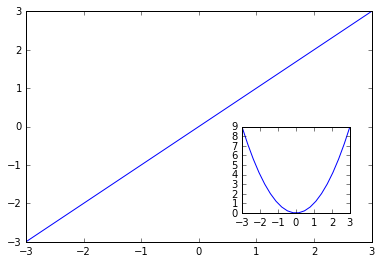
自由にグラフを配置する場合axesメソッドを使います。
|
1 |
axes([左, 下, 幅, 高さ]) |
各値を 0 から 1 の小数で指定します。
|
1 2 3 4 5 6 7 8 9 10 11 12 13 |
x = np.linspace(-3, 3, 20) y1 = x y2 = x ** 2 fig = plt.figure(figsize=(6, 4)) plt.axes([0.1, 0.1, 0.8, 0.8]) plt.plot(x, y1) plt.axes([0.6, 0.2, 0.25, 0.3]) plt.plot(x, y2) plt.show() |
描画はこうなります。
gridspec
グリッド上に変則配置
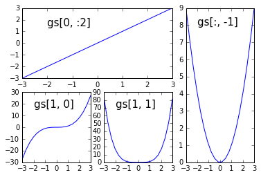
GridSpecを使うと、グリッド上で変則的な配置が行えます。
|
1 2 3 4 5 6 7 8 9 10 11 12 13 14 15 16 17 18 19 20 21 22 23 24 25 26 27 28 29 30 |
import matplotlib.pyplot as plt import matplotlib.gridspec as gridspec import numpy as np x = np.linspace(-3, 3, 20) y1 = x y2 = x ** 2 y3 = x ** 3 y4 = x ** 4 plt.figure(figsize=(6, 4)) gs = gridspec.GridSpec(2,3) plt.subplot(gs[0, :2]) plt.plot(x, y1) plt.text(-2, 1.5, 'gs[0, :2]', size=15) plt.subplot(gs[:, -1]) plt.plot(x, y2) plt.text(-2, 8, 'gs[:, -1]', size=15) plt.subplot(gs[1, 0]) plt.plot(x, y3) plt.text(-2, 17, 'gs[1, 0]', size=15) plt.subplot(gs[1, 1]) plt.plot(x, y4) plt.text(-2, 70, 'gs[1, 1]', size=15) plt.show() |
ポイント
以下の記述で figure を 2 × 3 のグリッドに分割しています。
|
1 |
gs = gridspec.GridSpec(2,3) |
gs を 2 × 3 の 2次元配列と考え、グラフを配置したい場所を指定します。たとえば
|
1 2 3 |
gs[0, 0] ⇒ 左上 gs[0, :] ⇒ 1行目すべて gs[:, -1] ⇒ 最終列すべて |
この gs[x, x] を subplot に渡して座標軸を作成します。
|
1 |
plt.subplot(gs[:, -1]) |
描画はこうなります。
ひよこパイソン says:
パイソン超初心者です。
いちばんはじめのx^2のグラフを実行してみたところ、couldn't connect to display "localhost:0.0"とエラーが出てしまいました。何かダウンロードしなければならないものがあるのでしょうか。
管理人 says:
こんにちわ、ひよこパイソンさん。
もしかして X 環境でしょうか。
python というより、サーバー関係の設定のような気がします。
たとえば、こんなページは参考になりませんか。
http://d.hatena.ne.jp/sobasobasoba/mobile?date=20121231
匿名 says:
包括的に記載していただいていて、大変助かりました。
管理人 says:
匿名さん、コメントありがとうございます。
EggPython says:
Python初心者です。
わかりやすい記事ありがとうございます。
下記のように関数から複数のaxesを作成している場合に、関数外でaxesを指定してデータを追加することは可能なのでしょうか?
***********************************************
#————————-
def Graph_(fig0,データ):
fig1 = fig0.add_axes([0.1,0.3,0.8,0.8])
fig2 = fig0.add_axes([0.1,0.1,0.8,0.2])
fig1.plot(データ)
fig2.plot(データ)
#————————-
Fig0 = plt.figure()
Graph_(Fig0,データ)
#◀ここで関数内で作った「fig2」にデータを追加したい
***********************************************
教えていただけると幸いです。
管理人 says:
EggPython さん、こんにちは
戻り値を使います。
#————————-
def Graph_(fig0,データ):
fig1 = fig0.add_axes([0.1,0.3,0.8,0.8])
fig2 = fig0.add_axes([0.1,0.1,0.8,0.2])
fig1.plot(データ)
fig2.plot(データ)
return fig2 # 戻り値
#————————-
Fig0 = plt.figure()
f = Graph_(Fig0,データ)
f.plot(データ)
EggPython says:
お返事ありがとうございます。
下記コードで実行してみたのですが、
※1の箇所で「AttributeError: 'NoneType' object has no attribute 'plot'」とエラーが出ます。
生成される上下2段のグラフのうち、上段の方(fig1)に(x,y3)のデータを関数の外で追加する方法をご存知であれば教え頂けると助かります。
そもそもfigureは作成後に編集するような操作はできないものなのでしょうか。
因みに※1か所を
plt.plot(x,y3)
とすると、下段のグラフ(fig2)にデータが追加されます。
よろしくお願いいたします。
==================================
import matplotlib.pyplot as plt
def Graph_(fig0,x,y1,y2):
fig1 = fig0.add_axes([0.1,0.3,0.8,0.8])
fig2 = fig0.add_axes([0.1,0.1,0.8,0.2])
fig1.plot(x,y1)
fig2.plot(x,y2)
#データの配列作成
x = [i for i in range(100)]
y1 = x
y2 = [i**2 for i in x]
y3 = [99**2-i**2 for i in x]
#グラフ描画
Fig0 = plt.figure()
f = Graph_(Fig0,x,y1,y2)
f.plot(x,y3)#・・・※1
==================================
管理人 says:
回答をよく見てください。
大事な1行が抜けちゃってます。
戻り値を fig1 にすれば上段に表示されます。
匿名 says:
すいません。
見落としていました。
ありがとうございました!
匿名 says:
非常にわかりやすいです!
助かりました!!